|
|
Linear regression with SAS
Linear regression overviewLinear regression model is a method for analyzing the relationship between two quantitative variables, X and Y. If the relationship between two variables X and Y can be presented with a linear function, The slope the linear function indicates the strength of impact, and the corresponding test on slopes is also known as a test on linear influence. On the other hand, if a linear model is used to fit relationship between X and Y, the stronger X and Y are linearly associated, the better fit the model for the date, and the corresponding test on strength of lindear association is also known as a test on linear correlation. The demonstration exampleSuppose in a health screening, seven people take measurement on Gender, Height, Weight and Age. The data is "measurement.csv". Open the data set from SAS. Or import with the following command.
  data measurement;
	infile "H:\sas\data\measurement.csv" dlm=',' firstobs=2;
	input gender $ height weight age;
    run;
Analyzing the impact of one variable on the otherIf the question is to investigate the impact of one variable on the other, or to predict the value of one variable based on the other, the general linear regression model can be used. In the demo example, if one wants to see impact of height on weight, or predict weight according to a certain given value of height. The model is Weight (continuous) ~ Height (continuous) We run regression model as follows. proc Reg data=measurement; title "Example of linear regression"; model weight = height; run; Reading the output of the linear regression
  				Example of linear regression

                                        The REG Procedure
                                          Model: MODEL1
                                   Dependent Variable: weight

                             Number of Observations Read           7
                             Number of Observations Used           7


                                      Analysis of Variance

                                             Sum of           Mean
         Source                   DF        Squares         Square    F Value    Pr > F

         Model                     1          11880          11880      84.45    0.0003
         Error                     5      703.38705      140.67741
         Corrected Total           6          12584


                      Root MSE             11.86075    R-Square     0.9441
                      Dependent Mean      155.57143    Adj R-Sq     0.9329
                      Coeff Var             7.62399


                                      Parameter Estimates

                                   Parameter       Standard
              Variable     DF       Estimate          Error    t Value    Pr > |t|

              Intercept     1     -592.64458       81.54217      -7.27      0.0008
              height        1       11.19127        1.21780       9.19      0.0003
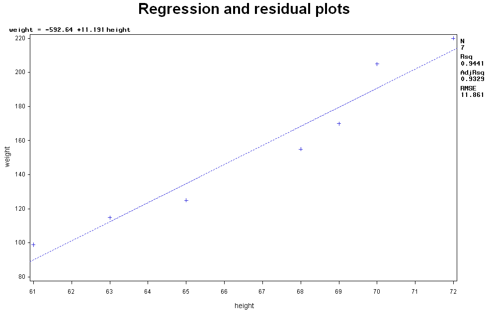
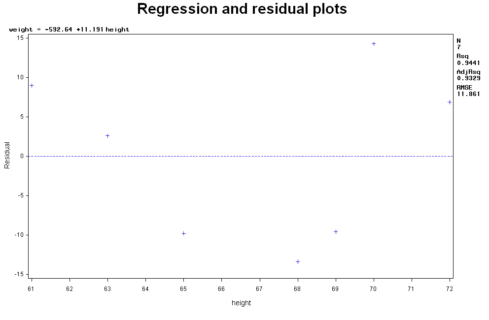
Interpreting the result of the linear regressionLinear regression assumes that the dependent variable (e.g, Y) is linearly depending on the independent variable (x), i.e., Y= β0 + β1(X) + random error, where β0 is the intercept and β1 is the slope. The output shows the parameters of β0 and β1 respectively, i.e, weight= -592.64458 + 11.19127*height + random error. Therefore, one can predict weight given height using this linear function between the two variables. For example, the predicted weight of a 70-inch-tall persion is -592.64458 + 11.19127 X 70=190.66 lbs. Furthermore, under the heading "parameter Estimates" are columns labeled "standard error","t value," and "Pr > |t|". The T values and the associated p-value test the hypothesis that the parameter is zero, or in other words, whether the (linear) effect of height on weight is zero. In this case the p-value is 0.0003, therefore we can conclude that the height has a significant linear effect on weight. Checking assumptions for the linear regressionLinear regression assumes that the relationship between two variables is linear, and the residules (defined as Actural Y- predicted Y) are normally distributed. These can be check with scatter plot and residual plot. You can also ask for these plots under the "proc reg" function. For example proc reg data=measurement; title "Regression and residual plots"; model weight=height; plot weight * height; plot residual. * height; output out=myout r=resid; The two plots are shown here:
From the residual plot you should check:
	proc univariate data=myout normal;
	qqplot resid /Normal(mu=est sigma=est color=red l=1);
	run;
As shown below the p-value for normality check is 0.3544, so the residuals are Normally distributed. Shapiro-Wilk W 0.903764 Pr < W 0.3544 Use data transformation to remedy the lack of normal assumptions.The convex shape of residual plot suggests that a second-order term (X2) might improve the model. So we introduce a quadratic variable, height2, and then fit a quadratic relationship between height, height2 and weight. The sencond-order variable height2, denoted as height2, can be created in the proc data, as shown below. Use data transformation to remedy the lack of normal assumptions.
	data measurement2;
		infile "H:\sas\data\measurement.csv" dlm=',' firstobs=2;
		input gender $ height weight age;
		height2 = height**2;
		run;

 	proc reg data=measurement2;
		title "Regression and residual plots with quatratic term";
		model weight=height height2;
		plot residual. * height;
		run;
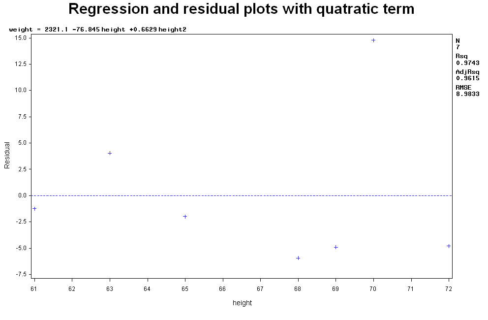
The resulting residual plot is given below. The distribution of residual is more random than the earlier plot. Note that when making conclusions on transformed data, one must conclude on the original variable, i.e., investigate the original variable by transforming it "back". Analyzing the correlation between two variablesSuppose the question is to find the linear association between every two variables, for example, Height and Weight, Height and Age and Weight and Age. proc corr data=measurement; title "Example of correlation matrix"; var height weight age; run; Reading the output of the correlation
                                 Example of correlation matrix


                                       The CORR Procedure

                            3  Variables:    height   weight   age


                                       Simple Statistics

   Variable           N          Mean       Std Dev           Sum       Minimum       Maximum

   height             7      66.85714       3.97612     468.00000      61.00000      72.00000
   weight             7     155.57143      45.79613          1089      99.00000     220.00000
   age                7      31.71429      11.42679     222.00000      20.00000      48.00000


                            Pearson Correlation Coefficients, N = 7
                                   Prob > |r| under H0: Rho=0

                                      height        weight           age

                        height       1.00000       0.97165       0.86467
                                                    0.0003        0.0120

                        weight       0.97165       1.00000       0.92621
                                      0.0003                      0.0027

                        age          0.86467       0.92621       1.00000
                                      0.0120        0.0027
Interpreting the result of the correlationProc Corr gives some descriptive statistics on the variables in the variable list along with a correlation matrix. The correlation is the top number and the p-value is the second number. For example, "height" and "weight" are highly correlatied with a correlation 0.9716 (with a p-value of 0.003). The small p-value (at a significant level of 0.05) suggests the correlation is significant. The matrix is symatric along the diagonal line. Note that an observed strong correlation between two variables does not necessarily indicate any causal connection between them, since the real causal variable might be hiddern or extrenous.
|
| © COPYRIGHT 2010 ALL RIGHTS RESERVED tqin@purdue.edu |


