|
|
Normality check procedure demonstrated with an exampleThe assumption of Normal distributionChecking the assumptionof Normality is necessary for many statistical methods. For example two sample t test or ANOVA. In this section we introduce some common ways to access normality: the normal probability plot and test statistics. The normal probabiltiy plot, QQplot creates quantile-quantile plots and compares ordered variable values with quantiles of a specific theoretical distribution. If the data distribution matches the theoretical distribution, the points on the plot form a linear pattern. In SAS, there are four test statistics for detecting the presence of non-normality, namely, the Shapiro-Wilk (Shapiro & Wilk, 1965), the Kolmogorov-Smirnov test, Cramer von Mises test, and the Anderson-Darling test. Details and discussions are given below. For example, in the two sample t test example , the assumption is the variables are normal. The data set is “reading.csv”. Method and intepretationUse the following syntax to load data and create QQplot. data read; infile "H:\sas\data\reading.csv" dlm=',' firstobs=2; input method $ grade; run; When a SAS data file "read" is created, the proc UNIVARIATE is used below to create QQplots and test statistics for accessing Normality. proc univariate data=read normal; qqplot grade /Normal(mu=est sigma=est color=red l=1); by method; run; Program note:
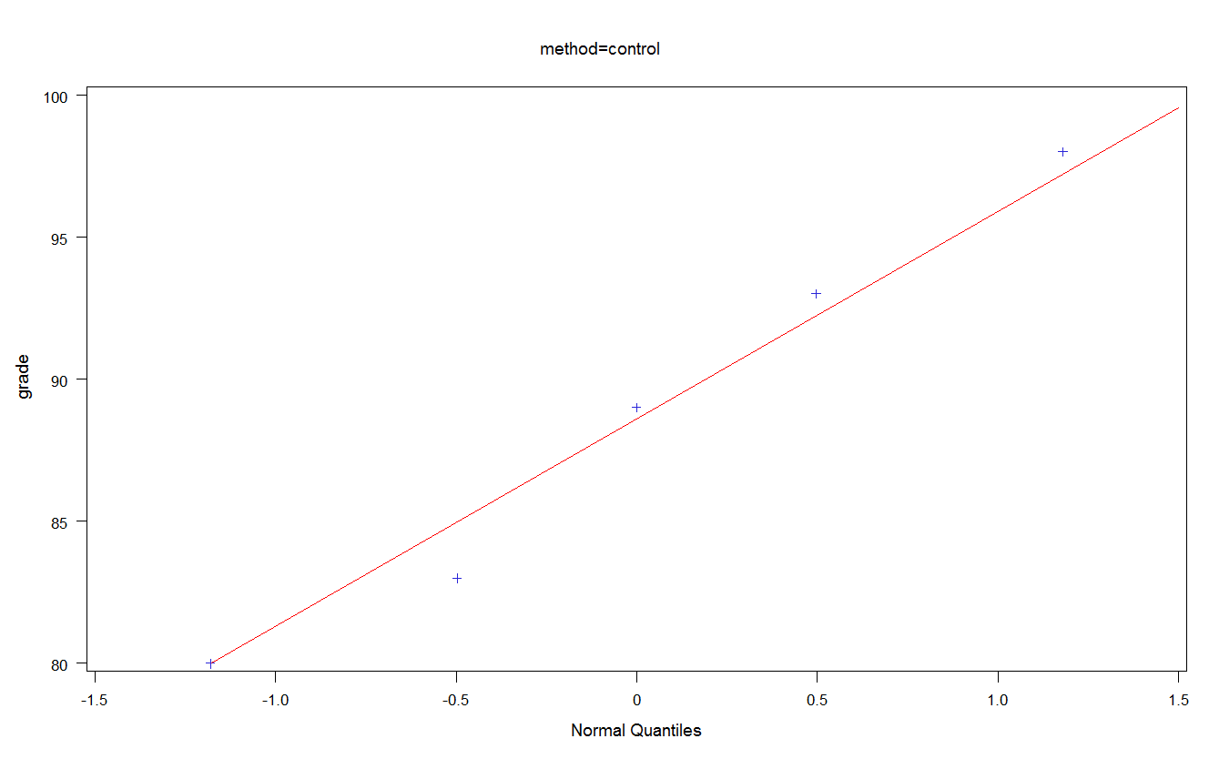
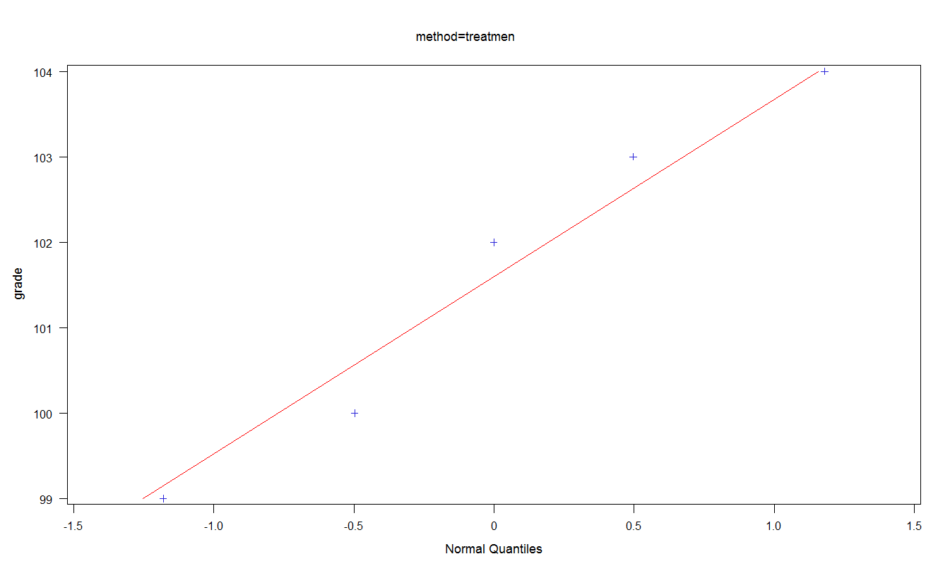
The QQ plots are shown here:
The QQ plots appear linear.Furthermore, the tests for Normality is given for both control and treatment group.
		Tests for Normality for Control Group

    Test                  --Statistic---    -----p Value------

    Shapiro-Wilk          W     0.969518    Pr < W      0.8721
    Kolmogorov-Smirnov    D     0.178474    Pr > D     >0.1500
    Cramer-von Mises      W-Sq   0.02439    Pr > W-Sq  >0.2500
    Anderson-Darling      A-Sq  0.172464    Pr > A-Sq  >0.2500
        Tests for Normality for Treatment Group

    Test                  --Statistic---    -----p Value------

    Shapiro-Wilk          W     0.952351    Pr < W      0.7540
    Kolmogorov-Smirnov    D     0.179821    Pr > D     >0.1500
    Cramer-von Mises      W-Sq  0.031987    Pr > W-Sq  >0.2500
    Anderson-Darling      A-Sq  0.206799    Pr > A-Sq  >0.2500
According to the SAS manual, if the sample size is over 2000, the Kolmgorov test should be used. If the sample size is less than 2000, the Shapiro test is better. The null hypothesis of a normality test is that there is no significant departure from normality. When the p is more than .05, it fails to reject the null hypothesis and thus the assumption holds. Since the sample size is very small and Shpiro test shows a big p-value of 0.8721 and 0.7540 respectively, it suggests that the data follows Normal distribution. |
| © COPYRIGHT 2010 ALL RIGHTS RESERVED tqin@purdue.edu |

